Multi‑Task Optimization over Networks of Tasks
 2 TH Köln
PPSN · 2026
We introduce MONET (Multi‑Task Optimization over Networks of Tasks), a multi‑task algorithm that represents the optimization state as a graph over tasks: each task is a node, each node stores its current best solution, and edges connect similar tasks so that knowledge can flow between them. MONET matches or exceeds MAP‑Elites-basd baselines across four benchmark domains (archery, arm, cartpole, and hexapod), scaling to 5,000 tasks on archery / arm / cartpole and 2,000 tasks on hexapod.
What does MONET look like?
At the core of MONET is a labeled graph $\mathcal{G}=(\mathcal{V}, \mathcal{E}, \mathcal{A})$, where nodes are tasks, edges are k-NN task‑space similarity, and each node is labeled with the best solution found so far.
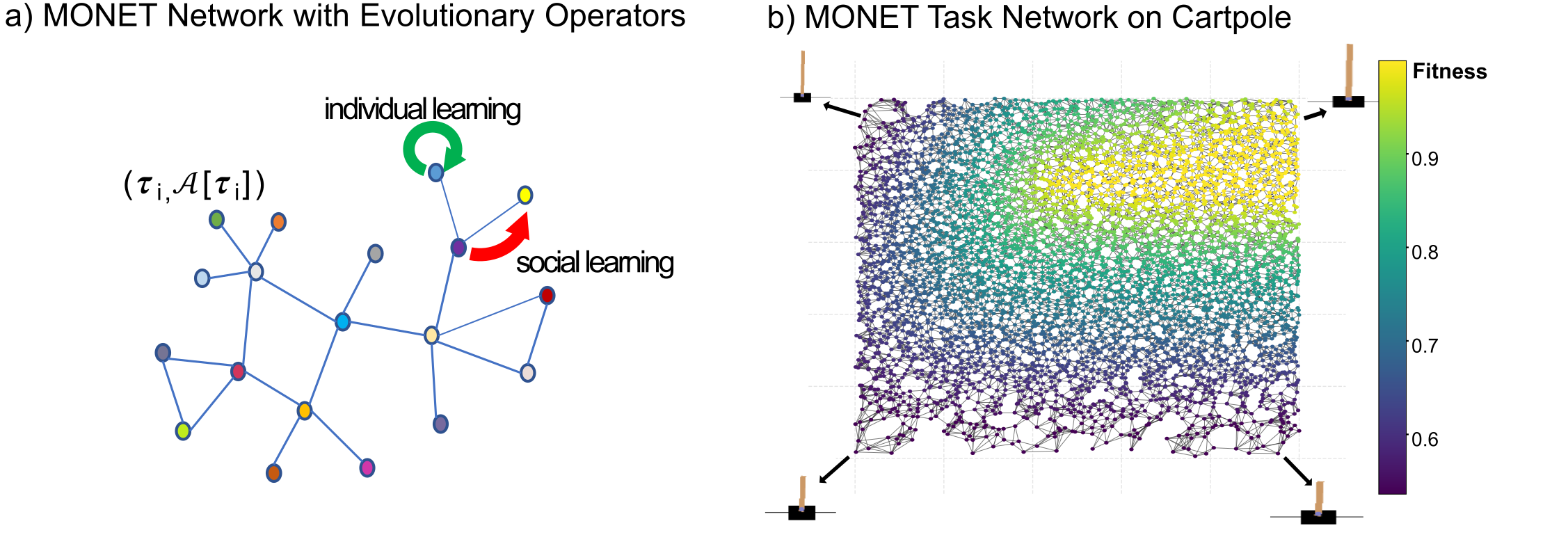
(a) Each node $V_i = \boldsymbol{\tau}_i$ is a task storing its current elite $\mathcal{A}[\boldsymbol{\tau}_i]$. Individual learning mutates a node’s own solution; social learning recombines a node’s elite with one drawn from its graph neighborhood. (b) The same task network mid‑run (500k / 1M evaluations) on the cartpole benchmark: color encodes per‑task fitness, showing how high‑quality solutions propagate along the edges.
Why is this relevant?
Real robots and real systems rarely come in one fixed configuration. A legged robot may lose a limb, a modular robot may reconfigure itself, a manufacturing line may swap components. Every variant is a distinct task with its own optimal controller, and re‑learning each one from scratch is wasteful.
Multi‑task optimization can tackle all of these configurations simultaneously and in parallel. But existing methods face a scalability–structure tradeoff:
- Population‑based multi‑task EAs maintain a population per task and have not been shown to scale past 1000 tasks.
- MAP‑Elites derivatives such as Multi-Task MAP-Elites (MT-ME, Mouret & Maguire, GECCO 2020 / arXiv:2003.04407) and Parametric-Task MAP-Elites (PT-ME, Anne & Mouret, GECCO 2024 / arXiv:2402.01275) do scale to thousands of tasks, but flatten the archive and mostly discard the topology of the task space: any elite can parent any task, regardless of similarity. While this could increase diversity, it might also decrease the likelihood of successfull knowledege transfer.
On top of that, classical MAP‑Elites pays a dimensionality tax. Fixing a common symbol: let $n$ be the number of task anchor points (grid cells, Voronoi cells, or graph nodes $\vert \mathcal{V}\vert$, depending on the method) in a $d$‑dimensional task space:
| archive | size scales as | task adjacency |
|---|---|---|
Grid-based (c bins per axis, d‑D tasks) | $\mathcal{O}(n)$ with $n = c^{\,d}$ forced | implicit, cell‑local |
| CVT-based ($n$ Voronoi cells) | $\mathcal{O}(n)$, $n$ chosen freely | reconstructed via Delaunay triangulation |
| MONET k‑NN task graph ($\lvert\mathcal{V}\rvert = n$ nodes, k edges/node) | $\mathcal{O}(n\,k)$, $n$ chosen freely | explicit graph edges |
We use the same $n$ across all three rows, so the comparison is at matched task‑space resolution. Under this lens, all three archives are $\mathcal{O}(n)$ up to MONET’s $k$ factor — the real dimensionality tax is not raw storage scaling but how $n$ is forced: grid-based MAP‑Elites couples $n$ to the task-space dimensionality via $n = c^{\,d}$, so reaching even $c = 10$ bins per axis in a $d = 10$‑D task space already demands $n = 10^{10}$ cells. CVT and MONET, by contrast, decouple $n$ from $d$, letting the practitioner choose the archive size directly. MONET pays an extra factor of $k$ (the number of edges per node, typically 1–5 % of $n$ in our experiments) on top of CVT’s raw cell storage, in exchange for explicit adjacency.
For $k \ll n$, MONET approaches the complexity of CVT, the regime we operate in, with many tasks and a fixed, comparatively small neighborhood. At the other extreme, $k = n$ yields a fully connected graph with $\mathcal{O}(n^2)$ storage.
While CVT archives (used by PT‑ME) sidestep the coupling of dimensionality and tasks by fixing the number of Voronoi cells for any dimensionality, the paid price is that adjacency is no longer a first‑class object (it has to be reconstructed via something like Delaunay triangulation) and local structure is collapsed into cell indices rather than preserved as a graph. Moreover, the way the centroids and impilicit neighborhoods are formed is fixed by CVT and not necessariliy the most useful for a given task space. MONET instead encodes task adjacency directly as graph edges, and closes this gap by making the task‑space neighborhood a first‑class structural element of the search.
How does it work?
An explicit graph over tasks. Given a task set ${\boldsymbol{\tau}_1,\dots,\boldsymbol{\tau}_n} \subset \mathcal{T}$ and a task distance $d$ (e.g. Euclidean), MONET builds a $k$‑NN graph in $\mathcal{T}$: each task points to its $k$ nearest neighbors, and these edges are the only channels along which knowledge can flow between tasks.
The variation operators we use are standard mutation and SBX crossover. What changes is who recombines with whom. We borrow nomenclature from cultural evolution to draw the line cleanly: a solution either improves in isolation, or by leveraging knowledge from another task.
Individual vs. social learning. At every step MONET picks a focal task $\boldsymbol{\tau}_i$. With probability $p_{\text{ind}}$ it applies individual learning, mutating $\mathcal{A}[\boldsymbol{\tau}_i]$ in isolation, exploring the task’s local landscape. Otherwise it applies social learning: drawing a neighbor $\boldsymbol{\tau}_j \in \mathrm{Nb}(\boldsymbol{\tau}_i)$ and recombining $\mathcal{A}[\boldsymbol{\tau}_i]$ with $\mathcal{A}[\boldsymbol{\tau}_j]$ via SBX crossover, transferring information between similar tasks. The candidate is accepted into $\mathcal{A}[\boldsymbol{\tau}_i]$ by the usual elitist rule.
The diagram below summarizes how these pieces fit together as a set of maps between the spaces MONET works in, with MAP‑Elites shown alongside for comparison.
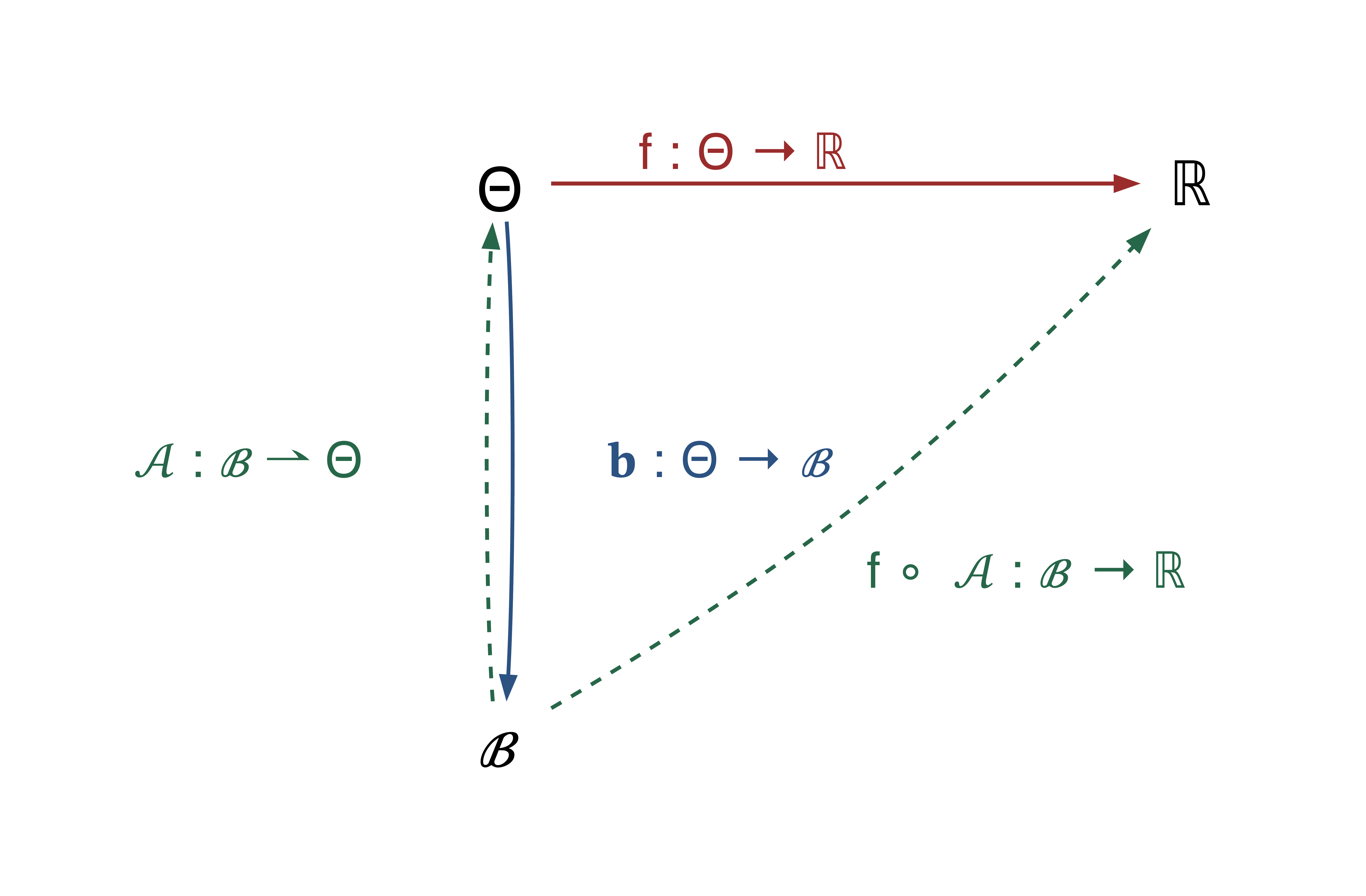
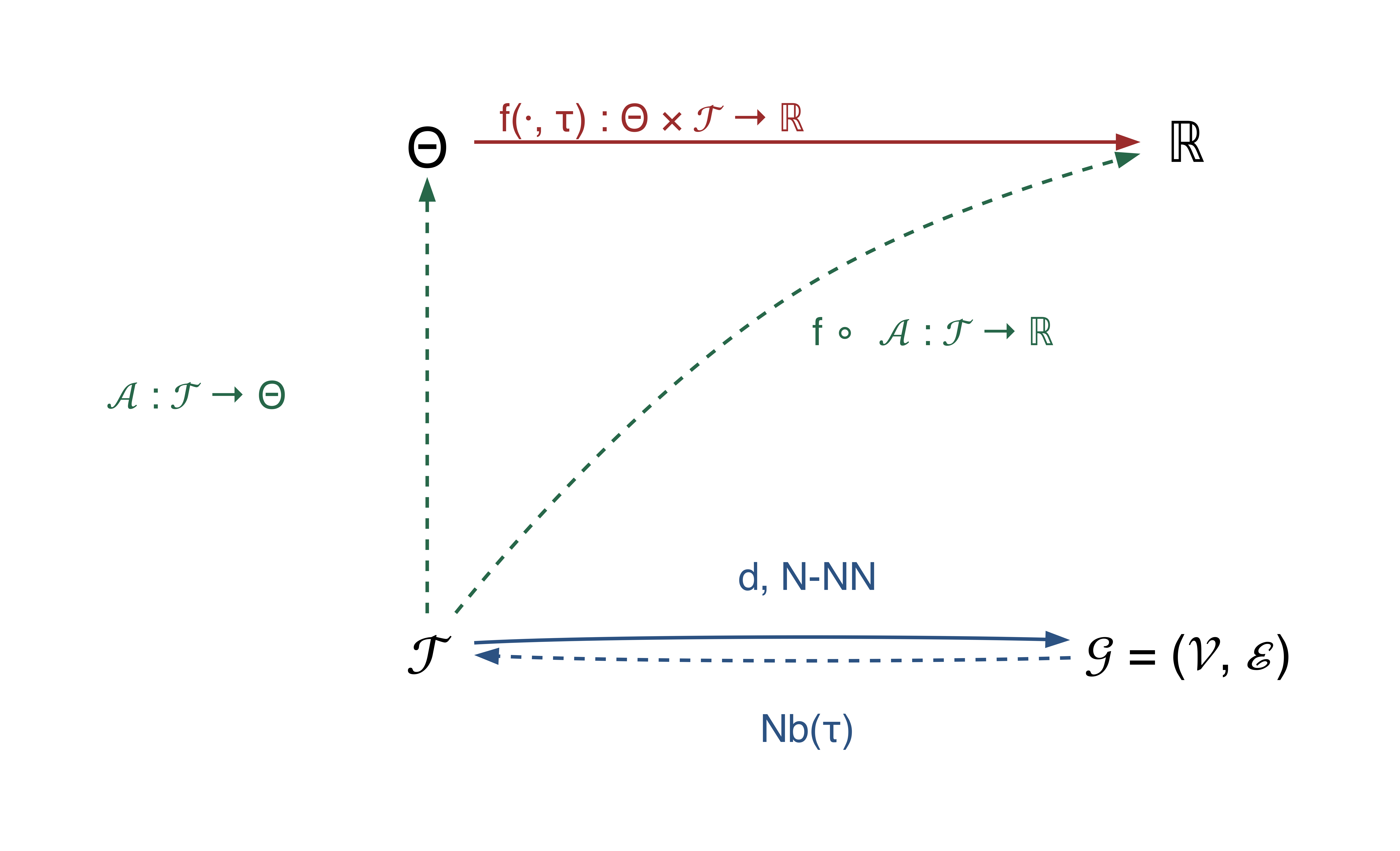
Read alongside MAP‑Elites, three changes stand out. First, the behavioral descriptor is gone: the archive is indexed directly by task, $\mathcal{A}:\mathcal{T} \to \Theta$, instead of by a hand‑designed descriptor. Second, fitness is task‑conditioned, $f(\cdot,\boldsymbol{\tau}):\Theta\times\mathcal{T}\to\mathbb{R}$ — the same controller can score differently on different tasks, so $\boldsymbol{\tau}$ has to appear as an argument. Third, the task distance $d$ and neighborhood lookup $\mathrm{Nb}(\boldsymbol{\tau})$ are explicit structural elements of the algorithm rather than artifacts of cell discretization; they are the channels social learning actually traverses.
Experiments
We evaluate MONET on four domains (archery, arm, cartpole with 5,000 tasks each; hexapod with 2,000 tasks) over a budget of $10^6$ evaluations, averaged over 20 seeds per (algorithm, domain) pair. Archery and arm report fitness in $[0,1]$; cartpole reports the mean balanced‑step count in $[0, t_{\max}{=}1000]$; hexapod reports the forward center‑of‑mass displacement in meters (in practice below $1.5\,\mathrm{m}$).
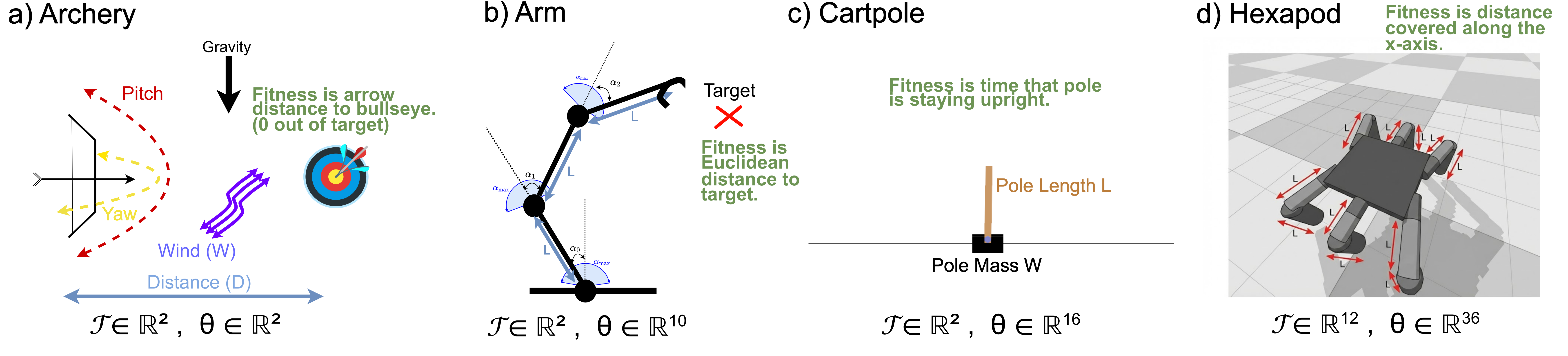
| Domain | Tasks | Task dim | Solution dim | Description |
|---|---|---|---|---|
| Archery | 5,000 | 2D | 2D | Projectile aiming under wind; tasks vary distance $D$ and wind $W$. |
| Arm | 5,000 | 2D | 10D | Planar arm reaches a target; tasks vary link length $L$ and max joint angle $\alpha_{\max}$. |
| Cartpole | 5,000 | 2D | 16D | NN‑controlled cartpole; tasks vary pole mass $m_p$ and length $L$. |
| Hexapod | 2,000 | 12D | 36D | hexapod locomotion; task = leg‑segment length changes. |
We compare MONET against two MAP‑Elites-based algorithms, MT‑ME (Mouret & Maguire, GECCO 2020 / arXiv:2003.04407) and PT‑ME (Anne & Mouret, GECCO 2024 / arXiv:2402.01275), reporting both a single shared default configuration (MONET$_{\text{default}}$) and per‑domain tuned configurations (MONET$_{\text{tuned}}$) obtained with the Sequential Parameter Optimization Toolbox (SPOT) (Bartz‑Beielstein, arXiv:2604.13672; SpotOptim on GitHub).
Results
MONET matches or exceeds the strongest MAP‑Elites baseline on every domain, with the biggest gap on hexapod, where the tuned configuration nearly doubles MT‑ME’s final fitness.
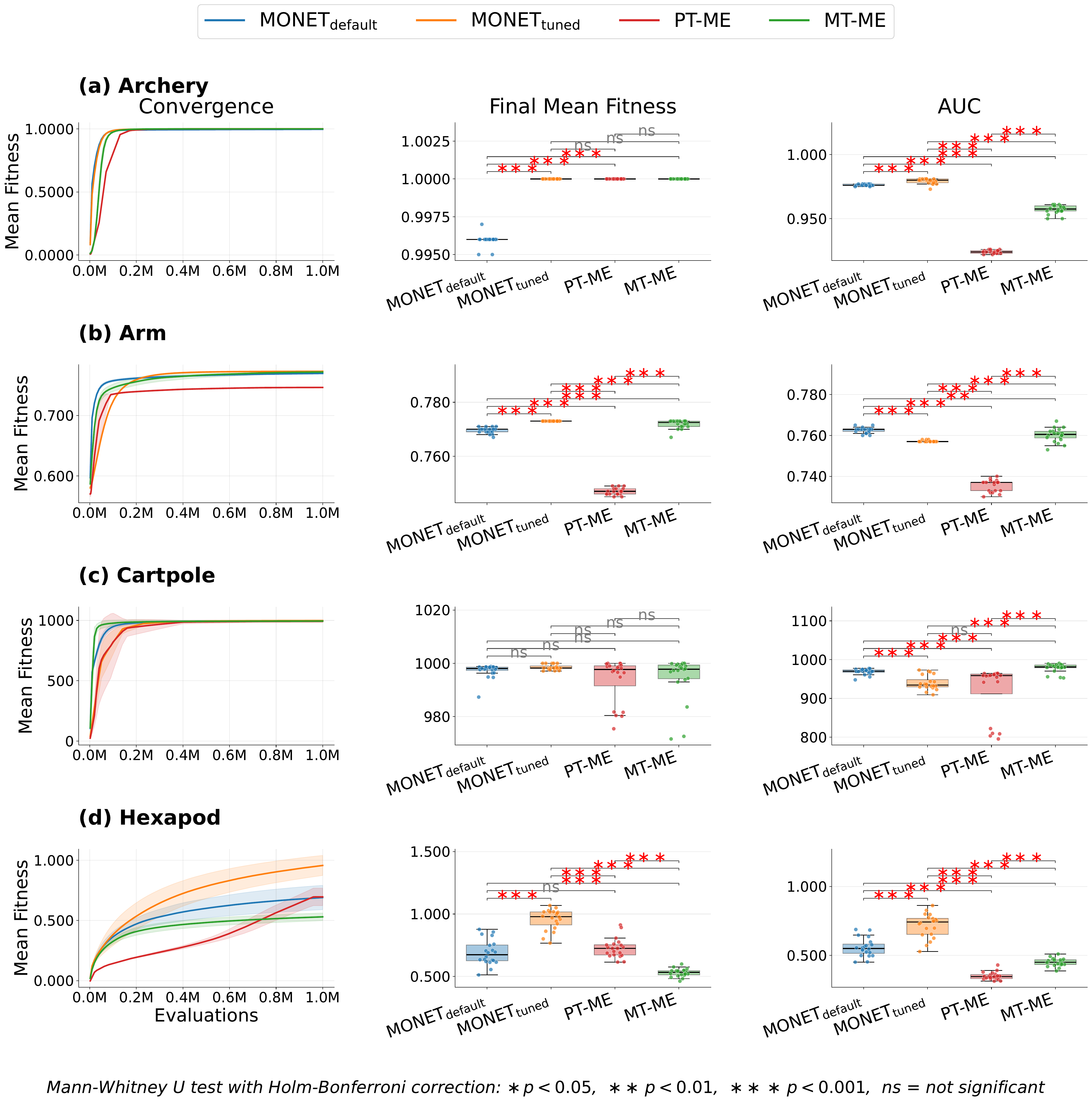
| Algorithm | Archery | Arm | Cartpole | Hexapod |
|---|---|---|---|---|
| PT‑ME | 1.000 ± 0.000 | 0.747 ± 0.001 | 992.5 ± 8.9 | 0.727 ± 0.078 |
| MT‑ME | 1.000 ± 0.000 | 0.772 ± 0.002 | 994.5 ± 8.5 | 0.530 ± 0.032 |
| MONETdefault | 0.996 ± 0.000 | 0.770 ± 0.001 | 997.2 ± 2.6 | 0.690 ± 0.101 |
| MONETtuned | 1.000 ± 0.000 | 0.773 ± 0.000 | 998.5 ± 1.0 | 0.957 ± 0.083 |
On archery, MONET reaches near‑optimal fitness substantially earlier than either baseline. On arm, MONET$_{\text{default}}$ ties MT‑ME on final fitness but leads on AUC (it converges faster). On cartpole all four methods come close to perfectly balancing the pole (final fitness between 997 and 998 out of a possible 1000), though MT‑ME still converges fastest on AUC. On hexapod, the domain with the most morphological heterogeneity, the graph‑aware routing pays off most: MONET$_{\text{tuned}}$ almost doubles MT‑ME’s final fitness.
Which hyperparameter matters?
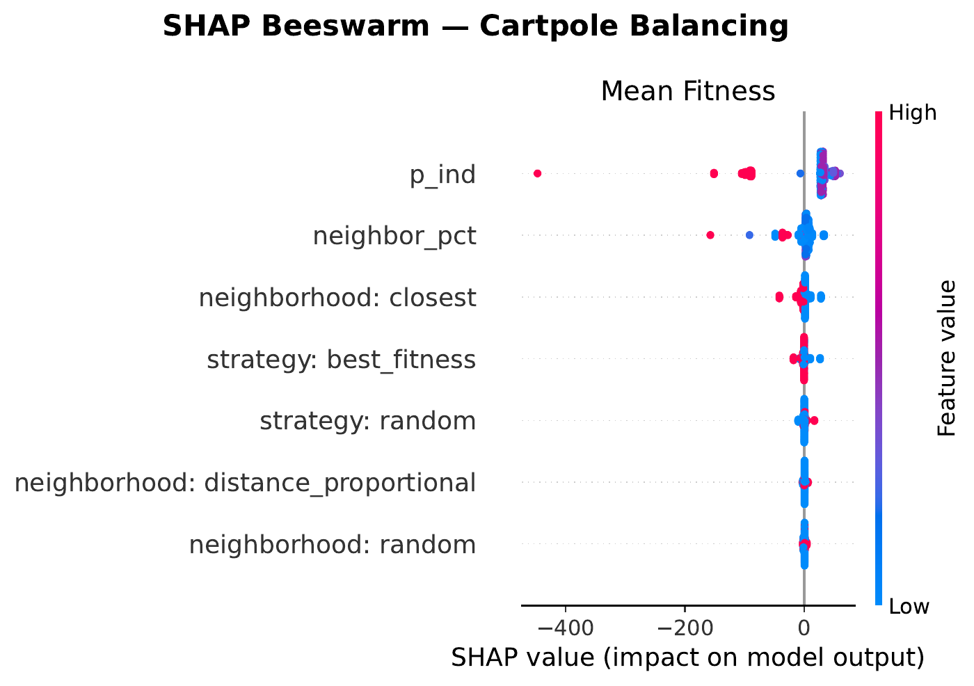
A SHAP‑based sensitivity analysis on a gradient‑boosted surrogate reveals that one hyperparameter dominates by an order of magnitude: the probability of individual learning $p_{\text{ind}}$.
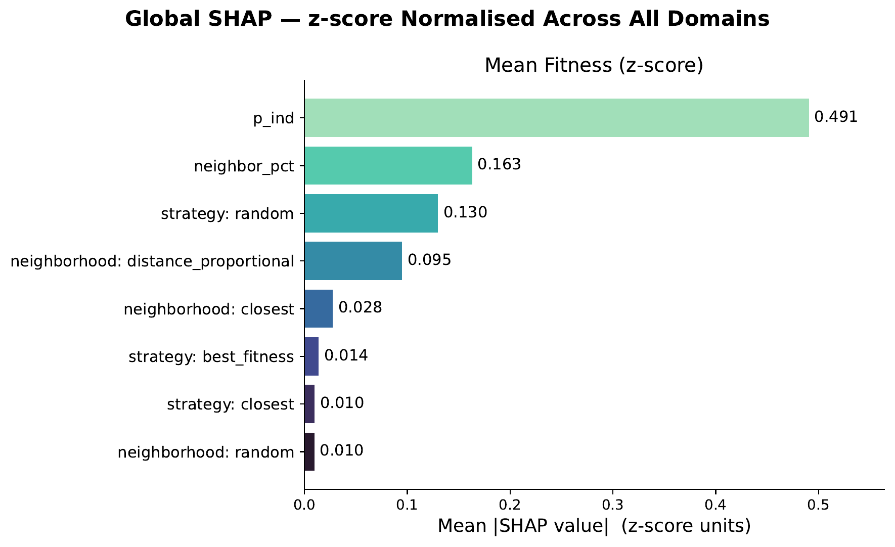
Lower $p_{\text{ind}}$ (i.e. favoring social learning over individual mutation) consistently improves both mean fitness and AUC across every domain. This directly supports MONET’s central design intuition: information transfer between similar tasks is the dominant lever in multi‑task optimization. The remaining hyperparameters (neighborhood type and size, selection strategy) show weaker, more domain‑dependent effects.
Per‑domain SHAP beeswarms
Zooming in on each domain, the beeswarm plots below show how each hyperparameter pushes or pulls the surrogate’s prediction of mean fitness (x‑axis is the SHAP value — negative means worse, positive means better — and color encodes the feature value from low to high). Each row is a hyperparameter; each dot is one MONET configuration in the sweep.
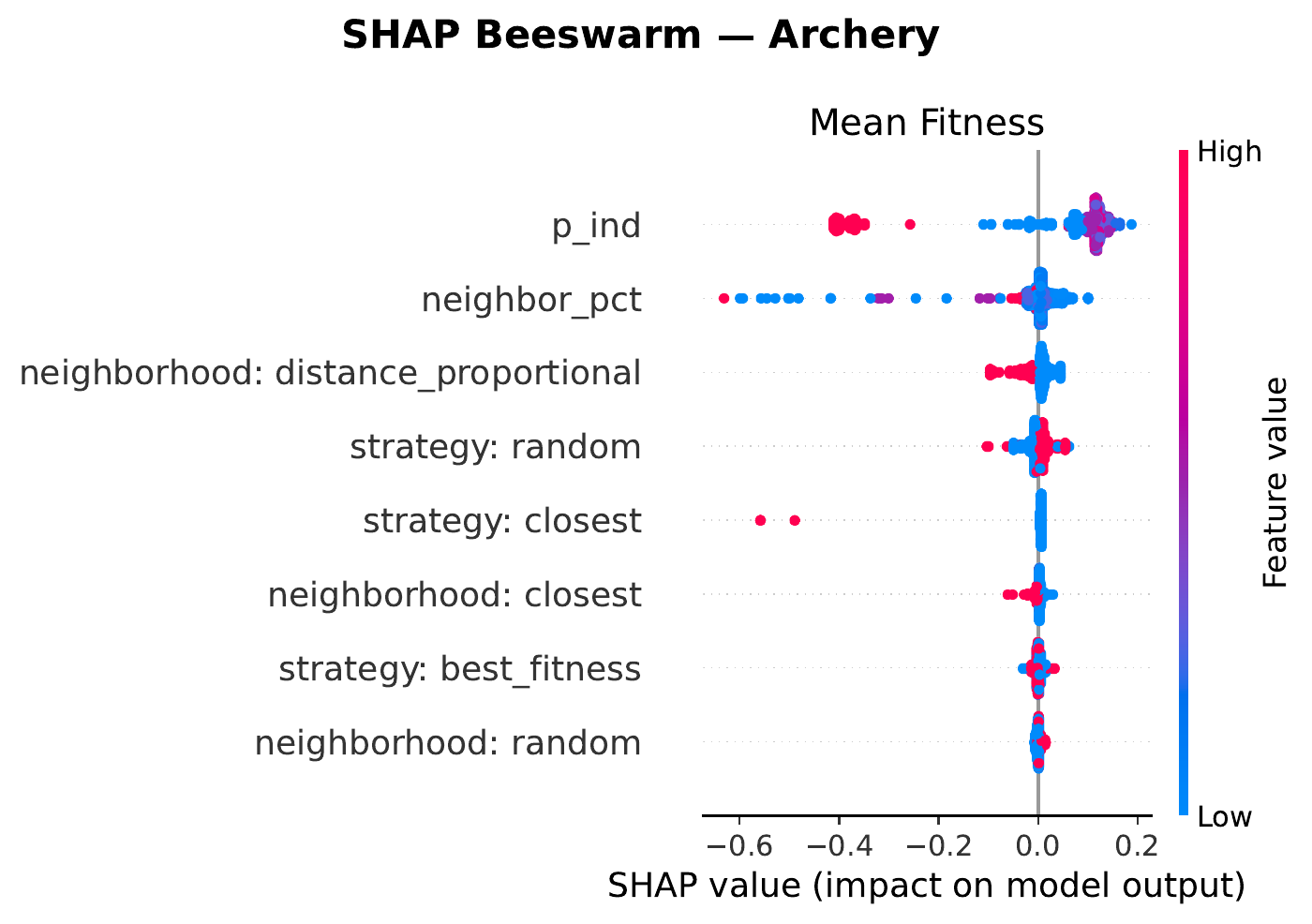
neighbor_percentage matters modestly; strategy / neighborhood are largely flat. SPOT‑tuned: $p_{\text{ind}}=0.22$ with a large neighborhood ($39\%$).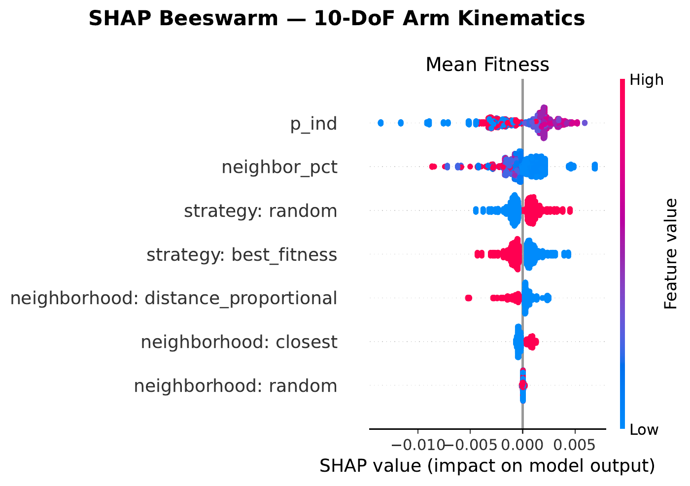
random neighborhood mode trend slightly positive.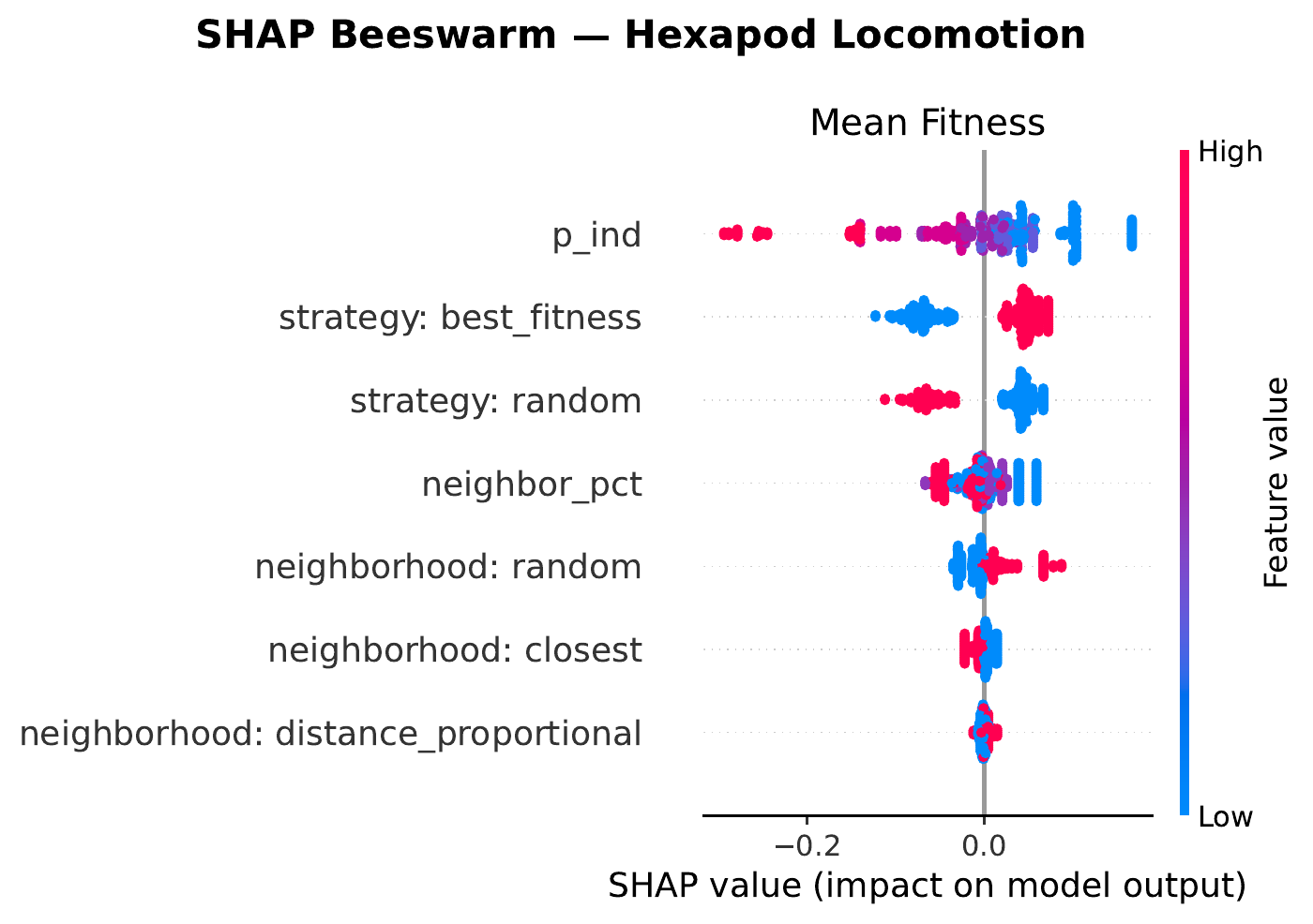
Two patterns hold across all four: (i) low $p_{\text{ind}}$ helps everywhere, with hexapod pushing the extreme to pure social learning ($p_{\text{ind}}=0$); and (ii) small neighborhoods (≤ 5 %) tend to outrank large ones, suggesting a benefit from keeping knowledge transfer fairly local in task space.
The default configuration we recommend is:
| Parameter | Default value |
|---|---|
p_ind | 0.3 (70 % social, 30 % individual) |
strategy | best_fitness |
neighborhood | closest |
neighbor_percentage | 5 % of tasks |
If you can afford per‑domain tuning, SPOT picks quite different optima on each benchmark — the tuned values that produce MONET$_{\text{tuned}}$ in the results above are:
| Parameter | Archery | Arm | Cartpole | Hexapod |
|---|---|---|---|---|
p_ind | 0.22 | 0.54 | 0.50 | 0.00 |
strategy | best_fitness | random | best_fitness | best_fitness |
neighborhood | random | closest | random | random |
neighbor_percentage | 39 % | 0.1 % | 1 % | 1 % |
The spread is telling: hexapod prefers pure social learning with a small neighborhood, arm tolerates almost no social learning at all on a very tight neighborhood, cartpole sits in the middle, and archery breaks the small‑neighborhood pattern — its fitness landscape is smooth enough that a large neighborhood of 39% still helps.
Ranking across the full sweep
Instead of tuning per domain, one can also ask: across the entire sweep, which MONET configurations generalize best, and which perform worst? We rank every configuration that was evaluated with at least 5 deduplicated seeds in every one of the four domains, by combined z‑score — the mean of the within‑domain z‑scores on final mean fitness. Eighteen configurations survive this coverage filter; the ten best and the five worst are shown below.
| strategy | neighborhood | nbr. % | $p_{\text{ind}}$ | $n_{\text{Arm}}$ | $n_{\text{Arc}}$ | $n_{\text{Cart}}$ | $n_{\text{Hex}}$ | $z_{\text{Arm}}$ | $z_{\text{Arc}}$ | $z_{\text{Cart}}$ | $z_{\text{Hex}}$ | combined |
|---|---|---|---|---|---|---|---|---|---|---|---|---|
| best_fitness | random | 1.0 | 0.00 | 40 | 39 | 12 | 20 | −0.29 | +0.57 | +0.42 | +2.33 | +0.76 |
| best_fitness | closest | 5.0 | 0.50 | 21 | 25 | 19 | 5 | +0.41 | +0.57 | +0.40 | +0.71 | +0.52 |
| best_fitness | closest | 5.0 | 0.30 | 21 | 29 | 21 | 20 | +0.17 | +0.56 | +0.41 | +0.87 | +0.50 |
| best_fitness | closest | 1.0 | 0.00 | 40 | 45 | 26 | 20 | −0.02 | +0.55 | +0.38 | +1.06 | +0.49 |
| best_fitness | closest | 1.0 | 0.50 | 40 | 44 | 26 | 5 | +0.70 | +0.57 | +0.40 | +0.06 | +0.43 |
| best_fitness | closest | 1.0 | 0.30 | 22 | 28 | 20 | 5 | +0.62 | +0.46 | +0.41 | +0.24 | +0.43 |
| best_fitness | closest | 10.0 | 0.50 | 20 | 24 | 19 | 5 | +0.17 | +0.57 | +0.40 | +0.32 | +0.36 |
| best_fitness | distance_prop. | 1.0 | 0.50 | 40 | 41 | 25 | 5 | +0.11 | +0.51 | +0.39 | +0.45 | +0.36 |
| best_fitness | closest | 5.0 | 0.70 | 20 | 20 | 20 | 5 | +0.51 | +0.57 | +0.37 | −0.03 | +0.35 |
| best_fitness | closest | 10.0 | 0.30 | 20 | 20 | 20 | 5 | −0.24 | +0.56 | +0.41 | +0.58 | +0.33 |
| strategy | neighborhood | nbr. % | $p_{\text{ind}}$ | $n_{\text{Arm}}$ | $n_{\text{Arc}}$ | $n_{\text{Cart}}$ | $n_{\text{Hex}}$ | $z_{\text{Arm}}$ | $z_{\text{Arc}}$ | $z_{\text{Cart}}$ | $z_{\text{Hex}}$ | combined |
|---|---|---|---|---|---|---|---|---|---|---|---|---|
| best_fitness | closest | 10.0 | 0.00 | 20 | 23 | 20 | 21 | −3.32 | +0.41 | +0.35 | +0.26 | −0.58 |
| best_fitness | distance_prop. | 1.0 | 0.00 | 40 | 41 | 27 | 20 | −2.39 | −0.35 | +0.34 | +1.50 | −0.23 |
| random | random | 1.0 | 0.50 | 40 | 39 | 25 | 5 | +0.49 | +0.56 | +0.35 | −0.78 | +0.15 |
| random | distance_prop. | 1.0 | 0.50 | 40 | 38 | 25 | 5 | +0.50 | +0.56 | +0.35 | −0.77 | +0.16 |
| random | closest | 1.0 | 0.50 | 40 | 39 | 25 | 5 | +0.78 | +0.57 | +0.34 | −0.76 | +0.23 |
Two patterns hold up under the stricter coverage filter. At the top, the closest neighborhood appears in 9 of the 10 best configurations and best_fitness task selection dominates all 10, while neighborhood sizes stay small (1–10% of tasks, mostly 1–5%) — consistent with the local-transfer view of MONET. The single best entry breaks the pattern only mildly: it uses a random neighborhood at 1%, so transfer is still local even if not strictly nearest. At the bottom, the random task-selection strategy resurfaces in three of the five worst entries, and the worst single entry is dragged down almost entirely by the arm domain ($z_{\text{Arm}} = -3.32$), where a 10% neighborhood with $p_{\text{ind}}=0$ destabilizes the search.
Conclusion
MONET suggests that task‑space topology carries information that flat, fully‑connected MAP‑Elites archives discard. Structuring the task set as a graph and routing recombination through graph neighborhoods gives a single, simple, scalable algorithm that matches or exceeds both MT‑ME and PT‑ME across four fairly different benchmarks. The gap is smallest on saturating tasks like archery and cartpole, where all methods converge to near‑optimal fitness, and largest on the most heterogeneous benchmark (hexapod), where the SPOT‑tuned variant roughly doubles MT‑ME’s final fitness.
Three directions open up next. First, edges can be drawn from signals other than Euclidean distance in $\mathcal{T}$, e.g. observed transfer success, or solution‑space similarity, to expose structure the parameter representation does not capture. Second, online self‑adaptation of $p_{\text{ind}}$, neighborhood size, and variation scales could remove the tuning burden. Third, richer social‑learning operators may strengthen transfer further on heterogeneous task sets.
BibTex
@misc{hatzky2026multitaskoptimizationnetworkstasks,
      title={Multi-Task Optimization over Networks of Tasks},
      author={Julian Hatzky and Thomas Bartz-Beielstein and A. E. Eiben and Anil Yaman},
      year={2026},
      eprint={2604.21991},
      archivePrefix={arXiv},
      primaryClass={cs.LG},
      url={https://arxiv.org/abs/2604.21991},
}
Correspondence
j.hatzky [at] vu [dot] nl
a.yaman [at] vu [dot] nl