Tanh Function as Drop-In Replacement for Layernorm
Reproduce these results: GitHub!
Do we really need LayerNorm?
LayerNorm is a widely used technique in modern deep learning models. It normalizes layer activations to maintain a consistent mean and variance across training data, stabilizing training and preventing issues like vanishing or exploding gradients.
Recently, Zhu et al., 2025 proposed a simpler and competitive alternative. They demonstrate that the tanh activation function can effectively replace LayerNorm in many cases. Their findings suggest that tanh offers comparable normalization benefits while improving computational efficiency and model simplicity.
The key insight is that LayerNorm’s input/output distribution often resembles an S-shaped curve, similar to that of tanh.
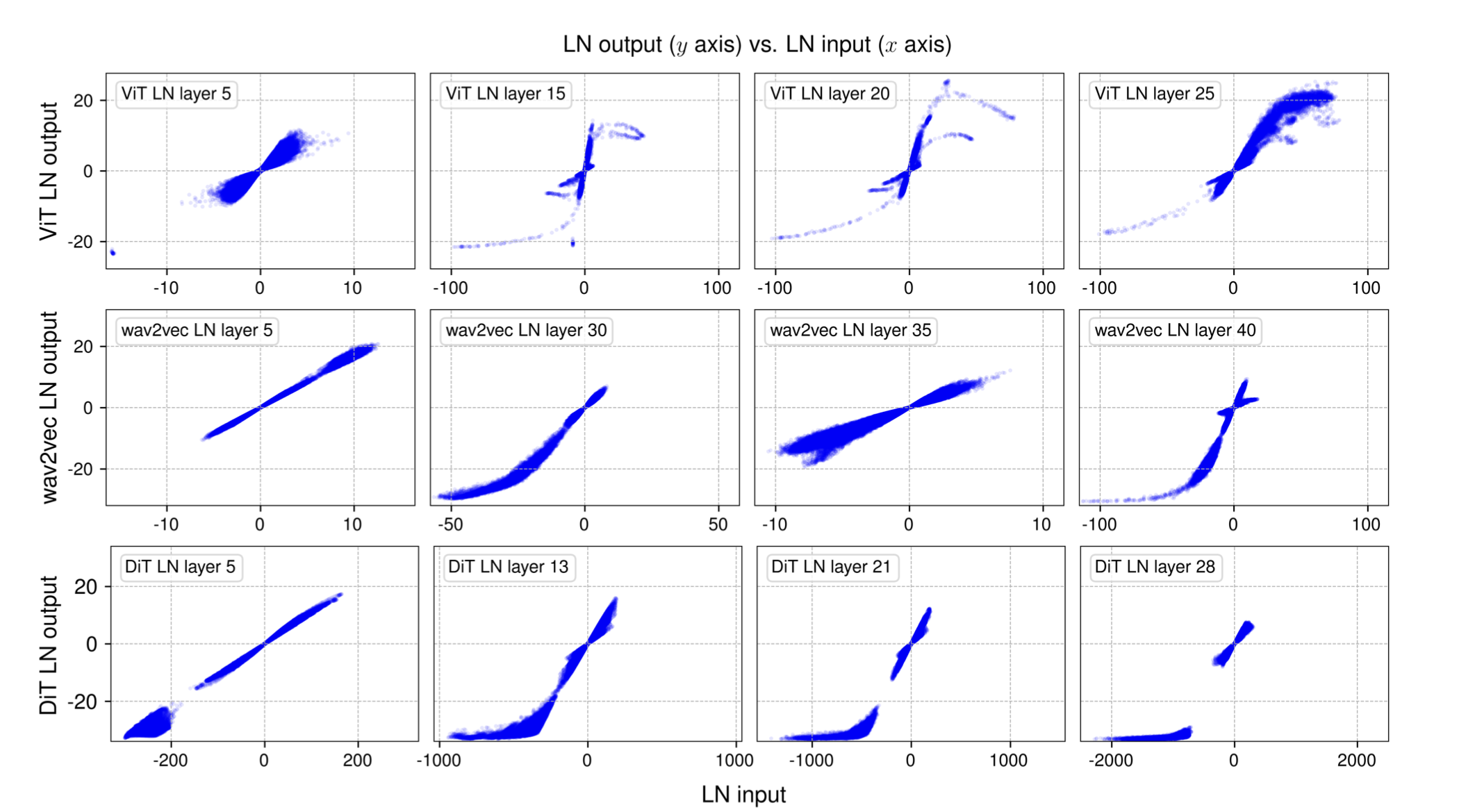
By using tanh as an activation function, the model inherently normalizes activations, reducing the need for explicit normalization layers. To increase flexibility, the authors introduce a learnable scaling factor, allowing the model to adjust normalization strength dynamically during training. They call this function Dynamic Tanh (DyT).
Why do we normalize?
One reason we need normalization layers like batch norm or layer norm is a well known problem called internal covariate shift (ICS).
ICS is the change in the distribution of network activations due to the change in network parameters during training. This can slow down the training process, as the network has to adapt to the changing distribution of activations at each layer. By normalizing the activations, we can ensure that the network sees a consistent distribution of activations at each layer, which can help to stabilize the training process and speed up convergence.
Even if the network is initialized so that the activations have zero mean and unit variance, the activations of the network will drift away from this distribution as the network is trained, making it harder to converge to a good solution. This observation is nothing new: for instance, it was reported by Yann LeCun in 1991.
LayerNorm vs. Tanh
Given an input tensor $x$ of shape $(B, C, H, W)$, the LayerNorm operation can be defined as:
\[\text{LayerNorm}(x) = \frac{X - \mu}{\sqrt{\sigma^2 + \epsilon}} \cdot \gamma + \beta\]where $\mu$ and $\sigma$ are the mean and standard deviation of $X$ respectively, and $\gamma$ and $\beta$ are learnable scaling and shifting parameters. The $\epsilon$ term is a small constant to prevent division by zero.
Calculating the mean and standard deviation of the input tensor can be computationally expensive, especially for large models and high-dimensional data. It typically is calculated over the spatial dimensions $(H, W)$:
mean = x.mean(dim=(2, 3), keepdim=True)
var = x.var(dim=(2, 3), keepdim=True)
which resembles a matrix multiplication operation with complexity of $O(B \cdot C \cdot H \cdot W) = O(N)$.
Now let us compare this with the parametrized tanh function (DyT):
\[\text{DyT}(x) = \tanh(\alpha x) \cdot \gamma + \beta\]where $\gamma$, $\alpha$ and $\beta$ are learnable scaling and shifting parameters. The tanh function is a simple element-wise operation, which is computationally efficient and can be easily parallelized on modern hardware. The scaling and shifting parameters can be learned using standard optimization techniques like gradient descent, making the DyT function a drop-in replacement for layernorm.
The complexity of the DyT function is $O(N \cdot C \cdot H \cdot W) = O(N)$, which is the same as the LayerNorm operation.
In summary, the computational complexity of both the DyT function and LayerNorm operation is $O(N)$, where $N$ represents the number of elements in the input tensor. However, when evaluating their efficiency on hardware, factors beyond theoretical complexity come into play.
LayerNorm requires multiple arithmetic operations: computing the mean $(O(N))$, variance $(O(N))$, and performing element-wise normalization $(O(N))$. These steps involve sequential reductions, which can introduce synchronization overhead and limit parallelism on hardware accelerators like GPUs and TPUs. Additionally, LayerNorm’s need to store running statistics can make parallelization more challenging.
In contrast, the tanh function is applied element-wise without dependencies, making it inherently parallelizable. This allows modern hardware accelerators to process all elements simultaneously, reducing synchronization overhead. Furthermore, tanh can be efficiently implemented using methods such as lookup tables or polynomial approximations, which significantly lower its computational cost.
Therefore, despite having similar theoretical complexities, the tanh function often demonstrates superior runtime efficiency in practical hardware deployments. This advantage is due to its minimal synchronization requirements, reduced memory overhead, and compatibility with modern accelerator architectures.
Experiment
Let’s run a small benchmark on the CIFAR-10 dataset to compare the DyT function with traditional LayerNorm.
We’ll train a simple convolutional neural network and measure the training time and accuracy of both normalization methods. To ensure a fair comparison, both models will start with the same weights and hyperparameters, differing only in the normalization layer.
Following the approach in the paper, we’ll first examine how the input and output distributions change after applying LayerNorm or the tanh-based alternative.
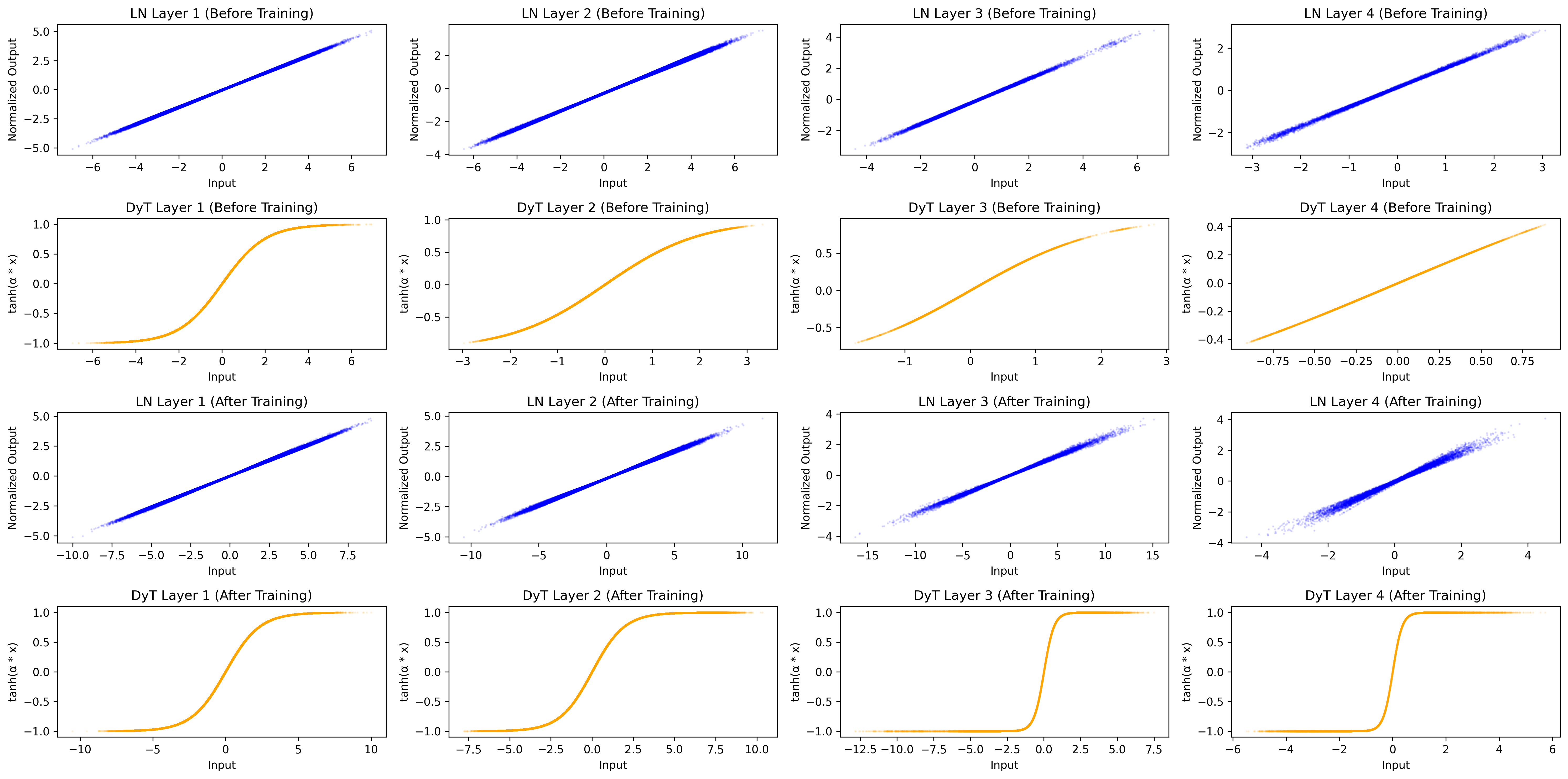
We can see, that the DyT is starting to become even stronger of an S-shaped curve. However, we can not observe this as clearly for the LayerNorm. Maybe it would occur after more epochs of training or with a different model architecture.
Next, we’ll train both models on CIFAR-10 for 100 epochs, tracking training and test loss.
As is visible, both models start to overfit pretty early on. However, the DyT model seems to generalize better and seems to have a lower divergence between training and test loss. While the learning dynamic is similar and can be tuned quite straight forward - for instance, we can introduce warmup, learning rate decay or dropout - there is something that is much harder to change: The computational efficiency of the tanh function compared to the layernorm operation. So let us take a look at the training and inference time of both models.
For the time, we measure the time it takes to complete one epoch on a single GPU. We repeat this process for 100 epochs and record the average training time per epoch.
In our small benchmark on CIFAR-10 we can make an obversation that is consistent with the authors: On average, the DyT model is faster to train than the LayerNorm model.
| Model | Training Time (s/epoch) | Inference Time (s/epoch) |
|---|---|---|
| LayerNorm | 25.52 | 15.44 |
| DyT | 23.77 | 14.51 |
| reduction | ↓ 6.9% | ↓ 6.4% |
Why do we get an increase in efficiency? This is due to the fact that the tanh function is a simple element-wise operation that can be easily parallelized on modern hardware, while the LayerNorm operation requires the explicit calculation of mean and variance, which can be computationally expensive. Definetly an argument for trying the DyT layer!
Reproduce the results here!
Cite This Article
@misc{hatzky2025dyt,
   title        = Tanh Function as Drop-In Replacement for Layernorm,
   author       = Julian Hatzky,
   year         = 2025,
   month        = Mar,
   url          = https://ju2ez.github.io/blog/2025/tanh/
}
Enjoy Reading This Article?
Here are some more articles you might like to read next: